Article written by Act-unity as part of their sponsorship ofACA Insurance Days 2022.
IFRS and IAS are accounting standards issued by the IFRS Foundation and the International Accounting Standards Board (IASB). One of the main goals of those standards is to standardize accounting standards to increase the comparability of companies, regardless of the country concerned. These standards are established by the IASB (International Accounting Standards Board) and must be validated at the European level for their application in the European Union.
In this context, the IFRS concerned becomes mandatory for the preparation of consolidated financial statements of listed companies. These standards are also mandatory for unlisted companies that issue or intend to issue listed debt securities. It should also be noted that some countries may allow these standards for the preparation of their corporate accounts.
Each IFRS Standard concerns a specific subject. The subject of this paper concerns IFRS 17 which concerns the mark-to-market valuation of insurance contracts (liability side) specific to insurance companies as well as the profit and loss account of insurance companies.
As IFRS17 is principle based, it does not give a clear method to compute the curve under which liabilities are discounted but, instead, it gives some principles which lead to some flexibility for entities. The aim of this paper is to provide an easy way to compute the IFRS17 discounting curve, relying on Solvency 2 quantities for European entities.
The interest rate curve is defined by paragraphs 36 and B72-B85 of IFRS17. The methodology for the discount curve construction is different than the one defined in the Solvency 2 framework. As the Standard is in nature a principle-based set of guidelines, a precise methodology of the discount curve construction is not outlined, rather a set of principles is provided. As such, this leaves some flexibility and judgements for its construction (paragraph B78). The chosen methodology should be disclosed together with all inputs, assumptions and estimation techniques used (collectively called as “significant judgements”) on every instance of IFRS 17 financial statements reporting (paragraph 117) and the curves shall meet the following criteria (paragraph 36):
According to paragraphs 36 and 33, the above criteria must be validated at the level of a group of insurance contracts (therefore an IFRS 17 discount curve is associated to a group of (re)insurance contracts). The main difference between the IFRS 17 curve and the risk-free interest rate curve defined by the Solvency 2 framework1 is the actual liquidity characteristic of the specific group of contracts that must be reflected by the IFRS 17 curve. The addition of a liquidity premium to the risk-free rates from Solvency 2 will result in higher rates under the IFRS 17 framework.
Two different approaches are described in the Standard: the bottom-up approach (paragraph B80) and the top-down approach (paragraph B81). The bottom-up approach consists in the addition of a liquidity premium of insurance contracts to a risk-free interest rate curve (RFR curve). This methodology is allowed unless cash-flows of insurance contracts vary based on the returns on underlying items.
The subject of this technical paper concerns the bottom-up approach. A good candidate2 for the risk-free interest rate curve is the RFR curve constructed by EIOPA for the Solvency 2 framework. So, the bottom-up approach could reuse some work already done for Solvency 2. Another possibility is to construct a liquid risk-free curve based on market data and on different assumptions than EIOPA’s (choice of the ultimate forward rate – UFR, duration of the liquid period and the speed of convergence of the curve to the UFR).
The liquidity premium needed for the application of the bottom-up approach shall reflect the illiquidity characteristic of specific insurance contracts. A possible methodology is to calibrate this amount on financial instruments with identical characteristics as the insurance contracts of the entity (lapses, volatility on the claims cash-flows in terms of date of payment as well as in terms of amount in case of claim…). As such, it could be difficult to find financial instruments with similar characteristics on the market. Our proposed methodology is based on a mark-to-model methodology instead of mark-to-market method.
The methodology can be summarized by the following formula3 :

The second part of the formula reflect the liquidity spread (computed on assets) corrected to reflect the liquidity of insurance contracts, that is where:
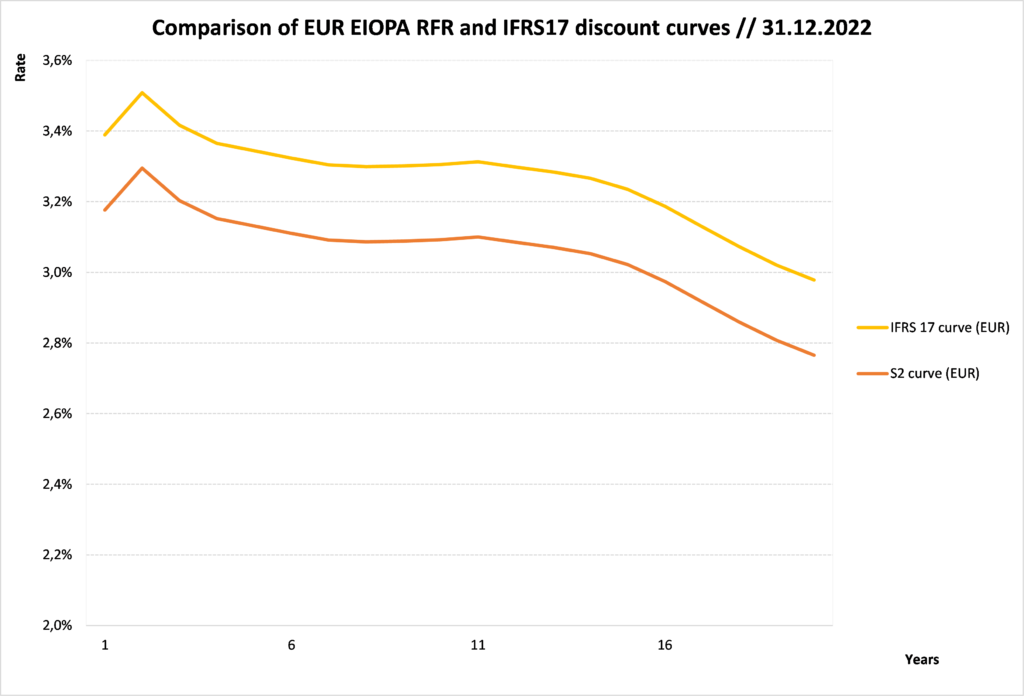
Based on a portfolio of contracts of duration 4 in EUR currency, the IFRS 17 curve based on the liability for remaining coverage at 31.12.2022 obtained by this methodology is illustrated in the following graph.
1Let us mention that the EIOPA curve is assumed to be consistent to the definition of risk-free rate curve under the Standard IFRS 17.
2If we accommodate to the assumptions from EIOPA in its construction of the RFR curve: choice of the ultimate forward rate (UFR), duration of the liquid period and speed of convergence of the curve to the UFR.
3The adequacy of the term DurA ⁄ DurP / 65% could be interpreted as a replacement of the factor 65% (which represents the difference of durations between assets and liabilities generic portfolios) but could also be demonstrated using a Taylor expansion.
The liquidity premium construction explained above (and so the resulting IFRS 17 discounting curve) is based on the reference asset portfolio of the EIOPA and not on the asset portfolio of a specific entity. As non-life insurance products are not directly backed by assets (unlike for life insurance contracts) and the overall impact on the Best Estimate is not assumed to be material, this approach reasonably reflects the reality and reduces the volatility adjustment coming from discount curve assessments between individual IFRS 17 financial statements reporting (because it is not dependant on modifications of asset portfolio from entities). Moreover, the sole reliance on a typical EIOPA generic portfolio (interpreted as a general portfolio of insurers) allows for a standardized price for non-life insurance contracts (in accordance with paragraph 36).
As already mentioned, the risk-free yield curve of the bottom-up approach (paragraph B80) could be chosen as the RFR curve from the Solvency 2 framework. The market consistency of this curve could be questioned because of the assumptions used for its calculation by EIOPA (i.e. the choice of the ultimate forward rate, the last liquidity point, the convergence point and the convergence tolerance used by the EIOPA). However, these assumptions only impact the curve for durations greater than 20 years. In case of long duration business (like savings products), we suggest calibrating the RFR curve on a longer LLP or evaluate the impact of this methodology in a specific study.
This approach is dependent on assumptions and methodologies applied by EIOPA. If EIOPA were to review the methodology used for the RFR curve or the VA calculation, an impact analysis would have to be carried out and the method should possibly be adapted (for information, a review of the VA and the RFR discounting curve is planned in the coming years following the review of the delegated regulation). However, one can believe that such modifications are occasional and infrequent and do not constitute a sufficient argument not to apply the pragmatic method explained. Moreover, the review of the delegated regulation is expected to be more market consistent than it is today.
The methodology developed in this paper gives an easy way to compute the IFRS17 curve based on quantities computed by EIOPA under the Solvency 2 framework. The number of stored information and computations is quite limited thanks to the few parameters needed for this process. Moreover, this method has advantages for the following reasons:
However, the drawbacks are the following:
The Act-unity team remain at your disposal for any questions or requests on the subject.
[2] International Accounting Standards Board, IFRS 17 Insurance Contracts, May 2017

2 minutes
Events, Tax & regulatory

10 minutes
Tax & regulatory

1 minute
Events, Tax & regulatory